The calibraton of the University of North Dakota's King Probe requires the determination of three calibration coefficients: C, x, and a.  The first step is to create a plot of King Probe voltage versus true air speed.  The best way to get the data for this plot is to take a dry run during a flight.  During this run the plane must fly out of cloud and vary its airspeed, preferrably anywhere between 60 and 140 m/s, while maintaining a constant pressure altitude.  After the data points for the plot are obtained the calibration program entitled "king_calib" is used to calculate the calibration coefficients.

The subroutine accepts arguments passed from the command line that include the start and end times of the calibration data during the flight, the analog file name, the winds file name, and the physical file name for that flight.  After the data is read in by the program it uses a curve fit function to find the best fit the data.  The program fits a function of the from .                                                   (1)

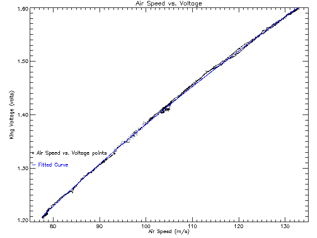
The best fit curve for this data is:  .                                        (2)  This gives x = .441 and a = -.254.  The constant C is the only variable left to determine.  It is determined by starting with the dry term of the King power:   ,                                     (3)  where Pdry is the power supplied to maintain a constant temperature in dry (out of cloud) air, Ts is the temperature of the sensor, Ta is the ambient air temperature, p is the atmospheric pressure, and v is the air speed.  Because the fitted curve does not pass through the point [0,0] a correction term, A, must be added to the equation because the fitted curve suggests that when the velocity is zero the voltage, and subsiquently the power, is not zero.  Therefore, the new form is:  .                                 (4)  The term A happens to be 10 times the term a, making it -2.54.  Since                                                          (5)  and the terms before v^x in (4) are all constants the dry term can be rewritten as:  .                                             (6)

Dividing through by 10 then yields: ,                                                (7)  where  ,   (8) and .                  (9)  This happens to be the fitted curve equation.  Therefore, the term K is known and the equation:                                    (10)  can be solved for C, which is the final constant to be determined.  Solving for C yields:  .                                (11)  From this run the term C is calculated to be 6.30e-4.

 This calibration procedure should be done after any repair, change, or service to the instrument.  Any work done to the instrument may greatly change the calibration coefficients.  Also, the constants should be verified at the start and end of every field project.  The values may not be exactly the same but it should be checked to see that any difference is negligable.

 Continue to Offset Correction page

 Back to Main page